A truck plant runs three systems that each believe they know when a chassis moved. The historian holds what the equipment did, at one-second resolution and heavily compressed. The ERP holds what was planned, ordered and billed. The floor itself — gate cameras, dock scanners, the weighbridge — holds what was actually observed. All three are telling the truth about something slightly different, and none of their timestamps agree. Joining process data to material flow is therefore a time problem before it is a data problem, and the compression that makes the historian affordable is exactly what makes the join delicate — because a value you ask for between two stored points is computed, not recalled. Request the integration datasheet.
Three Systems Know When the Chassis Moved. None of Them Agree.
Time alignment, sampling, compression and retention for joining plant historian data to vehicle material flow — and where a stored value stops being evidence and becomes an estimate.
Three Kinds of Truth About One Vehicle
Before any schema question, it is worth being clear about which system is authoritative for what.
Torque, current, pressure, flow, temperature, cycle state, machine availability, inspection results and alarms, arriving continuously as appends and almost never edited.
The order, the material master, the cost, the document numbers. Authoritative about intent and about money, and indifferent to the second at which anything physically happened.
A chassis through the gate, a trailer on a dock, a finished unit onto a transporter. Evidence with a timestamp and a photograph behind it.
The common architectural mistake is asking one of these to be authoritative for all three. An ERP document time is a perfectly good record of when somebody confirmed a transaction and a poor record of when a vehicle physically left. A historian tag is excellent evidence of a process condition and says nothing about which chassis was under the tool. Neither failing is a defect; both become one when a report treats them as interchangeable.
Where the Clocks Diverge
Here is the same chassis across a shift, on all three tracks.
The historian writes continuously whether or not anything interesting is happening. The ERP produces three documents across the whole shift. The floor produces four physical observations. The marked gap is the one that causes arguments: the unit was observed leaving through the gate twenty-eight minutes before the goods issue document was posted. Both timestamps are correct. They are answers to different questions, and a dispatch-performance report that silently picks one of them is reporting on the posting habits of the office rather than the movement of vehicles.
Compression Is Why the Value You Want May Not Exist
This is the part that most surprises teams coming from a transactional database background.
Swinging door trending maintains a tolerance corridor around the trajectory of a signal and writes a new point only when the signal would leave that corridor if the previous point were held. Related methods — a dead-band filter suppressing values within a tolerance of the last stored value, box-car, box-car with back-slope — work on the same principle. Typical compression runs from ten to one up to fifty to one, with noisy high-frequency signals compressing least and slowly varying temperatures and flows compressing most.
The consequence for a join is precise. Ask the historian for the value at the moment a chassis passed a station and it will usually return one, interpolated between the points either side. That is exactly right for a trend line and exactly wrong for a record of what happened, because the number has been computed rather than recalled. If the figure is going into an evidential record, it needs either a stored point or an explicit note that it was derived.
Which timestamp is your material flow actually joined on?
On most plants the honest answer is whichever one was easiest to reach, chosen years ago by somebody who has since moved on. In thirty minutes we will map the three clocks against one vehicle through your own line and show where the joins are landing.
What the Volumes Actually Look Like
Worth having real figures in hand before a retention conversation, because the intuitions are usually wrong in both directions.
A reference deployment of fifty machines carrying two hundred signals each gives ten thousand tags. Sampled at one hertz, that produces roughly 27 GB a day uncompressed. Swinging door compression at a typical ten to twenty times reduction brings it to somewhere around 1.5 to 2.7 GB a day. At enterprise scale the same arithmetic reaches 500 GB a day, or on the order of 180 TB a year per customer before compression is applied.
Those numbers explain why a general-purpose relational database is the wrong tool here. It breaks at industrial scale through index bloat, insert latency under sustained high write rates, and the absence of time-series-specific compression. A historian adds specialised tag metadata management, tiered storage, and query engines that execute time-range scans in memory without loading full indexes.
The write pattern is the other half of the explanation. Readings arrive at a regular cadence as a continuous stream of appends, with few or no updates or edits to historical rows — a workload almost perfectly opposed to what a transactional schema is optimised for.
Retention, and the Number That Catches Automotive Out
Three tiers, and one compliance figure that tends to arrive late in the project.
Live investigation, yesterday’s shift, the defect somebody is arguing about right now
Trend work, model training, quarter-on-quarter comparison
Where the automotive retention obligation actually lives
Regulated environments under GxP typically require ten years. Automotive production governed by IATF 16949 requires fifteen. That is a long way beyond what a storage budget sized against the hot and warm tiers will have anticipated, and it is a requirement about the record rather than about the query performance — so it is satisfied by cold object storage rather than by anything expensive, provided somebody worked it out before the first archive policy was written rather than after.
Sampling, Downsampling and the Count Nobody Keeps
A small point with a large consequence for anyone training a model on this data.
Downsampling a raw measurement usefully produces more than one output. An average supports long-term trends. A maximum supports threshold analysis. And a count shows whether the interval contained the number of observations it was supposed to contain — which is the one most often dropped, and the only one that tells you whether the average is trustworthy.
Without it, an interval during which a gateway was offline looks identical to an interval during which the process was simply stable. Both produce an average. Only the count distinguishes a quiet machine from a dead sensor, which is the same distinction as a quiet gate and a camera that has silently stopped reporting.
Store-and-forward handles the outage itself correctly — data replays to the historian in chronological order with original timestamps preserved, and a multi-day gap can back-fill in the background with nothing lost. The risk is not the data; it is anything that queried that window before the back-fill arrived and cached the answer.
Where Oneflow Sits in This
Not as a replacement for either system. As the layer that records what was observed and files it where the business plans and bills from.
A camera at the gate, a scanner on the dock, a weighbridge. The physical event happens and is captured with its own time.
A reading the system is not sure of is never quietly offered. It appears as held, with the reason attached, and cannot be selected.
Nothing is applied until a person presses the button. The record says who approved it and when.
Arrivals and dwell as transport documents, defects as maintenance notifications, odometer and tread as measurements against the asset, movements as stock movements.
The design rule behind all four steps is the one that matters for a data architecture: nothing is applied until a person presses the button, because a form that fills itself silently is one nobody trusts twice. That holds the evidential quality of the observation layer in a way an automatic write-back cannot — and it is also why ERP write-back is off by default, with a sandbox that builds the identical message and stops before the network so the bytes can be read before anything is live.
Six Ways These Joins Go Wrong
Each one produces a report that looks reasonable. Swipe the table sideways on mobile.
| Failure mode | What goes wrong and what to do instead |
|---|---|
| Joining on the wrong timestamp | The ERP document time is when somebody confirmed it, not when the chassis moved. Join material flow to the observation, and carry the document time as a separate attribute rather than as the clock. |
| Interpolating a compressed value into a record | The historian will happily return a value for a moment it never stored. That is correct behaviour for a trend and wrong behaviour for evidence. |
| Downsampling to an average and losing the count | An average over an interval hides a gap in it. Keeping a count alongside shows whether the interval contained the number of observations it should have. |
| Assuming clock discipline across the plant | Controllers, gateways, servers and cameras drift independently. A join at second resolution across undisciplined clocks is a join on noise. |
| Treating a back-filled gap as live data | Store-and-forward replays in order with original timestamps preserved, which is the right design — but anything that read the window before the back-fill arrived was reading an incomplete picture. |
| Letting retention be decided by storage cost alone | The cheapest answer and the compliant answer are rarely the same, and in automotive the compliant answer is measured in years, not months. |
How This Connects to the Vehicles Themselves
Everything above is about the plant. The same architecture continues past the gate, and the join problem goes with it.
A finished chassis leaving the line becomes an asset with its own measurement history — odometer, tread depth, defect records — filed against the asset rather than against a process tag. The signals change but the discipline does not: a measurement belongs to a specific unit at a specific time, with evidence behind it, and an uncertain reading is held rather than guessed. That is what makes a service schedule downstream something you can defend rather than something you maintain by hand.
It is also what makes predictive work honest. A model trained on historian data from the plant and condition data from the operating fleet is only as good as the alignment between them, and the alignment is only as good as the timestamps. The daily inspection record is the same kind of object as a historian tag — an observation, at a time, about a specific unit — and it belongs in the same architecture rather than in a separate system that has to be reconciled later.
How FleetRabbit Handles This
Four things, aimed at keeping the observation layer evidential rather than merely convenient.
The historian keeps the process truth and the ERP keeps the plan. What was observed on the floor becomes a third record with evidence behind it, rather than a number somebody retyped into one of the other two.
A value the system is not confident in is marked held with its reason and cannot be selected, because a guess in a system of record is worse than a gap.
The sandbox builds the identical message and stops before the network, so an integration lead can inspect exactly what would have been sent before anything is enabled.
Each step states plainly whether it runs on its own or is still done by a person, so nothing on the screen claims an automation it does not have.
Questions Plant IT Teams Ask
Why can we not just join on the ERP timestamp?
Because it records when a transaction was confirmed, not when a vehicle moved. In the example above those are twenty-eight minutes apart. Join material flow to the observation and carry the document time as a separate attribute. Check Your Join Keys.
Does historian compression lose data we need?
It loses points, deliberately, and keeps the shape of the signal within a tolerance you set. That is ideal for trends and a problem only when a specific stored value is needed as evidence, because the historian will interpolate rather than tell you it has nothing. Review the tolerance.
What compression ratios should we expect?
Typically ten to one up to fifty to one, depending on the signal. Noisy high-frequency signals compress least; slowly varying temperatures and flow rates compress most. Ten thousand tags at one hertz runs around 27 GB a day raw and roughly 1.5 to 2.7 GB a day compressed. Size it against your tags.
How long do we have to keep it?
Hot for roughly thirty days, warm out to about two years, and cold indefinitely. GxP environments typically require ten years; automotive production governed by IATF 16949 requires fifteen, which is the figure most often missed when the archive policy is written. Review Your Retention Tiers.
Why keep a count when we downsample?
Because an average hides a gap. A count tells you whether the interval contained the number of observations it should have, which is the only thing distinguishing a stable process from a sensor that stopped reporting. Add it to the pipeline.
What happens to data during a network outage?
Store-and-forward queues on site and replays in chronological order with original timestamps preserved, so a multi-day gap back-fills with nothing lost. The thing to watch is anything that queried and cached that window before the back-fill landed. See how captures queue.
Will this write back into our ERP automatically?
Not by default, and deliberately. Write-back is off until enabled, and the sandbox builds the identical message and stops before the network so you can read the real bytes first. Uncertain readings are held with a reason rather than sent. See the Ground Truth Layer.
Can the same approach cover vehicles after they leave the plant?
Yes, and it is the same object model — an observation, at a time, about a specific unit, with evidence attached. Measurements against an asset and defect records file the same way process data does. Start a Sandbox Connection.
Give the Plant a Record of What Actually Happened
Oneflow watches, records and files. The historian keeps the process truth, the ERP keeps the plan and the money, and what was observed on the floor stops being a number somebody retyped — held when uncertain, approved by a person, and filed as the document type it actually is.