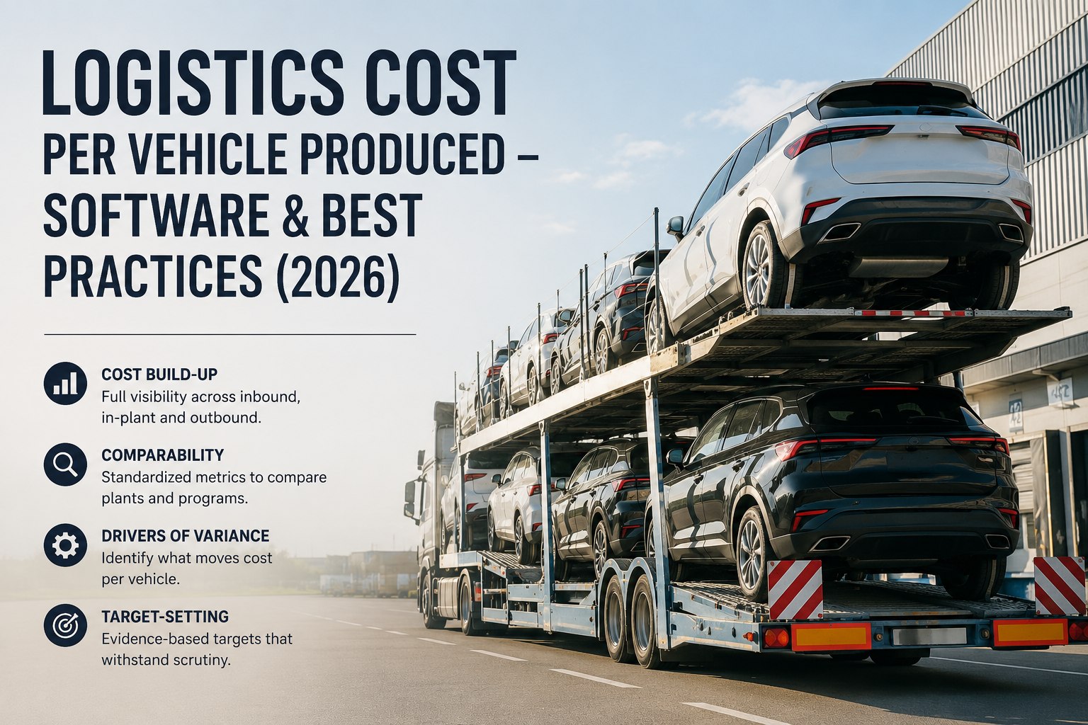
Logistics cost per vehicle produced is the number every OEM quotes and very few can defend under questioning, because it is a ratio and both halves of it are contestable. The numerator depends entirely on where you draw the scope boundary — inbound only, or in-plant handling, or packaging, or the premium freight that planning generated. The denominator depends on which vehicles you count and whether a three-variant plant and a twelve-variant plant are the same unit at all. Get either wrong and you have produced a figure that looks comparable and is not, which is worse than having no figure, because it will be used to set a target. What makes the effort worth it is the scale: automotive logistics constitutes around 8% of a vehicle's retail price, so a metric this size deserves a definition that survives a finance review. Book a 30-minute working session and bring last quarter's figure — we'll take it apart in Fleet Rabbit and show you which of your plants are genuinely comparable and which only look it.
2026 GUIDE · COST PER UNIT
Logistics Cost per Vehicle Produced
A cost build-up with a stated boundary, comparability rules that hold across plants, the drivers that actually explain variance, and target-setting that does not collapse the first time someone asks how the number was made.
≈8%Everything else in the retail price
Automotive logistics runs at roughly eight per cent of a vehicle's retail price. On flat production volumes, that share cannot be improved by selling more — only by measuring it properly and changing what drives it.
The Build-Up
Five layers, and the argument about your number is almost always an argument about which of them are inside the boundary. State the scope before quoting the figure.
L1Inbound transport
Freight to the plant across all modes, including drayage and terminal charges. The layer everyone includes, and the only one some plants include.
WatchPrepaid freight buried in part price is real cost sitting outside this line entirely
L2In-plant logistics
Gate, yard, dock, internal transport, line feed and sequencing labour. A distinct discipline with its own cost structure, and frequently sitting in a production overhead rather than a logistics one.
WatchWhether outsourced in-plant services are counted the same way as in-house labour
L3Packaging and containers
Returnable pool depreciation, cleaning, repair, replacement and expendable spend. Capital-heavy and easy to leave out because it is not an invoice arriving monthly.
WatchPool capital treated as capex at one plant and expensed at another
L4Premium and exception cost
Expedite freight, emergency packaging, abnormal handling. Include it — it is the layer that responds fastest to management attention, and excluding it flatters the plants with the worst planning discipline.
WatchWhether it sits in freight or gets absorbed into production recovery
L5Indirect and system cost
Software amortisation, administrative overhead and compliance — the layer most often skipped and the one that makes a cost framework complete rather than approximate.
WatchCentral costs allocated to plants on a basis nobody at the plants can reproduce
Why siloed data breaks the number
The data has to be pulled from procurement, warehousing, transportation and service functions together — and the more siloed it is, the harder it becomes to identify true cost drivers. That is not a reporting inconvenience; it is the reason plants produce figures that cannot be reconciled. Start with transportation spend, warehousing and inventory value, then layer the indirect costs on top rather than treating them as an afterthought.
The Denominator Is Not Simple Either
"Vehicles produced" sounds unambiguous and is not. Four decisions have to be identical across sites before any comparison means anything.
1Which units countUnits off the line, units shipped, or units saleable. Scrapped and reworked builds consumed logistics cost, so excluding them understates the numerator's true burden.
2Which periodCost incurred against units produced in the same window. Freight paid in one month for parts consumed in the next distorts a monthly figure badly and averages out only over a quarter.
3Complexity per unitA high-variant vehicle carries more parts, more sequencing and more packaging types than a low-variant one. Raw units treat them as equal, which is why complexity-adjusted comparison is the only fair version.
4Knock-down and partial buildsKits shipped for assembly elsewhere consumed inbound and packaging cost at your plant but did not become a vehicle there. Decide where they land, and apply it identically everywhere.
Bring two plants' figures to a 30-minute session
We'll put both through the same five-layer boundary in Fleet Rabbit and show you where they diverge — scope, denominator or genuine performance. In most groups it turns out to be at least two of the three, and knowing which one before the next cost review changes the conversation entirely.
Comparability Across Plants
Before comparing two sites, normalise for the things neither plant controls. Location factors and regional characteristics genuinely influence comparability, and so do volume, mix and seasonality — a differentiated approach is required rather than a single ranking.
← Swipe to see all columns →
The honest position is that a single cross-group league table is usually indefensible. What works is banded comparison plus trend — group plants by distance, volume and complexity, compare levels only inside a band, and compare movement over time across bands. That gives you a fair ranking and a fair improvement measure without pretending two structurally different plants are competing on the same terms.
What Actually Drives the Variance
Six drivers explain most of the gap between plants once the structural factors are normalised out. Five are controllable.
Premium freight rateThe single most responsive driver, and the one that most reflects planning discipline rather than logistics execution. A plant with double the expedite rate of its peers has a forecasting problem, not a freight problem.
Inbound consolidation levelPartial loads versus full loads across the same supply base. Consolidation quality varies enormously between plants nominally running the same network.
Container pool efficiencyCycle time and loss rate feeding pool size. A plant carrying a large buffer because it cannot see its assets is paying for uncertainty in this line every year.
In-plant handling intensityTouches per part between gate and line. Layout drives part of this and process discipline drives the rest, and only the second is comparable.
Yard and dock throughputDetention, dwell and waiting time absorbed into freight rates and internal labour. Invisible in the transport budget and very visible in the per-unit number.
Working capital policyLow inventory reduces holding cost and adds logistics complexity — a deliberate trade rather than a failure, and one that has to be read alongside the cost figure rather than through it.
Where the savings have to come from now
Rate pressure alone will not deliver the reductions being asked for in 2026 — cutting rates and headcount is not enough on its own, and a large share of cost elimination has to come from optimisation, process upgrades, and in some cases design and supply chain change. With mature-market production forecast to be broadly flat, the per-unit figure cannot be improved by volume either. That leaves the six drivers above as the realistic route.
Setting a Target That Survives Scrutiny
Six rules. Most targets fail on the first two, long before anyone questions whether the number was achievable.
1Publish the boundary with the targetWhich of the five layers are in scope, stated in the same document. A target attached to an undefined numerator will be met by redefining the numerator.
2Baseline before you commitA full rolling year on the agreed definition, per plant. Targets set from a benchmark rather than your own baseline are indefensible in either direction.
3Set it per band, not per groupPlants in different distance, volume and complexity bands should carry different targets. A uniform percentage across structurally different sites is a target nobody defends internally.
4Name the driver behind the numberA target of a given reduction should map to specific drivers — expedite rate, consolidation, pool efficiency — rather than being a percentage in search of a mechanism.
5Hold the definition still for the yearScope changes mid-year make the comparison meaningless. Version the definition and restate history if it has to change.
6Report level and trend togetherLevel answers where a plant sits; trend answers whether it is improving. Only reporting one produces either complacency or unfairness depending on which you chose.
What the System Has to Do
Five capabilities. Without them the figure is assembled by hand each quarter, which is why it changes shape every time somebody new assembles it.
One source of truth across functionsTransport, warehousing, packaging and premium spend in a single model rather than four exports reconciled in a spreadsheet. Siloed data is what makes true cost drivers hard to identify.
Scope boundary as a configurationLayers switched in and out to answer different questions from the same underlying data, with the active boundary stamped on every report.
Cost allocated to the driver eventFreight to the lane, premium to the cause, pool cost to the programme — so the per-unit figure decomposes rather than just totalling.
Complexity and volume normalisation built inBand membership held per plant, so comparison is automatic rather than a manual adjustment somebody has to remember to apply.
Rolling twelve-month view as the defaultBecause a single month is dominated by shutdowns, launches and timing effects, and the monthly view is where most misleading conclusions get drawn.
Half a day on your definition is worth more than a quarter on your rates
On a working session we'll take your current build-up, your plant list and one quarter of actual spend into Fleet Rabbit — set the five-layer boundary, band the plants, and produce a comparable per-unit figure alongside the decomposition that explains the gaps. You keep the definition document either way, and most teams find at least one plant that was being judged on a number it never owned.
Frequently Asked Questions
What should be included in logistics cost per vehicle?
Decide the boundary explicitly and publish it. A complete build-up runs to five layers: inbound transport, in-plant logistics, packaging and containers, premium and exception cost, and indirect costs including software amortisation, administrative overhead and compliance. Most published figures include only the first. The framework that works starts with total transportation spend, warehousing fees and inventory value, then layers the indirect costs on top — and pulls that data from procurement, warehousing, transportation and service functions together rather than one at a time.
Can we compare plants directly?
Only within bands. Location factors and regional characteristics genuinely influence comparability, and so do production volume, model mix and seasonality — which is why a differentiated approach is required rather than a single ranking. Group plants by supply base distance, volume and complexity, compare levels only inside a band, and compare trend across bands. A single cross-group league table looks decisive and is usually indefensible the moment someone asks how two specific sites were normalised.
How big is this cost, really?
Automotive logistics constitutes around 8% of a vehicle's retail price, which is why OEMs examine every part of the value chain for efficiencies and why cost pressure passes so directly to logistics providers. For a plant team the practical implication is that a metric of this size deserves a proper definition — an 8% cost line measured on an unstated boundary is not a controlled cost, it is an estimate that happens to be reported monthly.
Why does the denominator cause so much trouble?
Because "vehicles produced" hides four decisions: which units count — off the line, shipped or saleable — which period the cost is matched against, how complexity is handled, and where knock-down kits land. A high-variant vehicle consumes materially more logistics than a low-variant one, so raw unit counts flatter complex plants' peers and penalise the complex plants. Fix all four identically across sites, or accept that the comparison is directional at best.
Where do the savings come from if not rates?
Optimisation and process change. Cutting rates and headcount is not enough on its own — a large share of cost elimination has to come from optimisation, upgrades and process updates, and in some cases design and supply chain change. Practically that means premium freight rate, consolidation level, container pool efficiency, in-plant handling intensity and yard throughput. With mature-market production forecast to be broadly flat in 2026, spreading fixed cost over more units is not available as a route.
How do we set a target that holds up?
Publish the boundary with the target, baseline a full rolling year on that definition before committing, set it per band rather than uniformly across the group, and map the number to named drivers rather than issuing a percentage in search of a mechanism. Then hold the definition still for the year — scope changes mid-year make the comparison meaningless, and a target attached to a movable numerator will always be met by moving it.
Book a session with your current target and we'll stress-test it against your own baseline in Fleet Rabbit before it goes into next year's plan.
Define It, Then Defend It
Five layers with a stated boundary, a denominator settled on four explicit decisions, plants banded before they are compared, variance decomposed to named drivers, and a definition that stays still for a full year.
Bring last quarter's figure to the call · Works alongside existing ERP and TMS · Free tier available