Delivery frequency is the one inbound parameter that is almost never optimised and almost always inherited. Somebody set the milk run at twice a shift years ago, the line rate has changed twice since, container quantities have changed once, and the route still runs twice a shift because it always has. The reason it matters is that frequency sits at the intersection of two costs moving in opposite directions: reducing line-side inventory lowers holding costs, throughput times and internal material handling, and under lean thinking it also improves control over part quality and supplier performance while maintaining useful pressure on the system — but it simultaneously increases the frequency of milk-run routes and the number of suppliers on them, which raises transport cost. The empirical shape of that trade-off is what makes it tractable: transport cost rises only gradually as inventory is first reduced, which means there is a zone where you can take most of the inventory benefit before the transport penalty becomes serious. Ask for the deployment brief to find that zone for your own routes.
DESIGN GUIDE · INBOUND FLOW
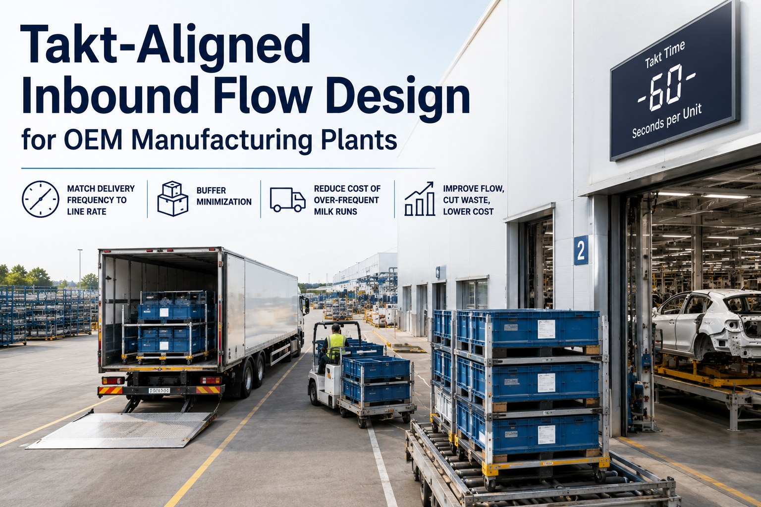
Takt-Aligned Inbound Flow Design
Delivery frequency matched to line rate rather than to history, buffers minimised without paying for it in transport, and the real cost of an over-frequent milk run made visible before it is committed.
DailyLarge buffers
2× shiftBalanced
4× shiftBalanced
HourlyTransport heavy
ContinuousTransport dominant
Where most of the inventory benefit is available at modest transport cost
Two Curves Moving in Opposite Directions
Frequency design is the search for the crossing zone between these two. Neither curve is linear, which is why intuition is a poor guide and why the answer differs by part family rather than being a site-wide policy.
As frequency rises
Line-side and plant inventory falls
Holding cost and working capital fall
Throughput time shortens
Internal material handling reduces as storage is eliminated
Quality and supplier problems surface faster, because there is less stock hiding them
The benefits are partly intangible and generally considered significant — which is exactly why they get asserted rather than quantified.
As frequency rises
More route departures per day
More suppliers added to each route to fill it
More stops, and handling cost is charged per stop
Lower load factor per departure
More dock slots, more gate transactions, more yard events
Transport cost rises only gradually as inventory is first reduced — the early moves are cheap, the later ones are not.
The point people miss
Because the transport penalty starts gently, there is usually a substantial reduction in inventory available before cost begins climbing meaningfully. Plants that never model this either stay where they are — assuming any increase in frequency is expensive — or overshoot into continuous replenishment and pay a transport bill that no inventory saving justifies. Both errors come from treating the relationship as linear.
What an Extra Run Actually Costs
Milk-run cost is a sum of components, and adding a departure does not scale all of them equally. Build it up rather than quoting a rate per kilometre, because the components behave differently and only some of them are avoidable.
Cost = fixed + (per-km × distance) + (driver wage × time) + (handling × stops) + inventory
Fixed costVehicle and overhead. Spread across cargo, which is why high utilisation matters — milk runs generally target loading factors above 85%.
Variable per kilometreFuel is usually the largest variable expense, driven by price, consumption and distance. Optimised routing and fuller loads reduce both burn and emissions.
Driver timePaid for time as well as distance, including waiting and loading — so congestion and dwell at stops feed straight into wage cost.
Handling per stopCharged per stop and often estimated around one minute per cubic metre. More frequent runs mean more stops carrying smaller quantities, so this component scales badly.
Inventory costThe component the other four are being traded against. Include it explicitly or the analysis will always favour fewer, larger runs.
Note what happens when frequency doubles: distance roughly doubles, driver time more than doubles once waiting is counted, handling scales with stops rather than volume, and load factor halves unless suppliers are added — which adds stops again. That is the mechanism behind the curve.
Frequency inherited from a previous line rate is the most common inbound cost left on the table.
The deployment brief covers frequency modelling per part family, the cost build-up per route, and how consumption data feeds a frequency that tracks takt instead of tradition.
Setting Frequency Per Part Family
Frequency should be determined by consumption pattern and supplier lead-time reliability, not applied uniformly. These are the inputs that move the answer, and the direction each one moves it.
← Swipe to see all columns →
The last row is the one that turns a logistics decision into a site decision. Every added run is a gate transaction, a dock slot and a yard event — so a frequency increase that looks cheap on transport can be expensive at a gate already operating near its throughput limit, where waiting climbs disproportionately rather than proportionally.
Symptoms of Over-Frequency
Too many runs fails less visibly than too few, because nothing stops. It shows up as cost and congestion rather than as a shortage, which is why it persists for years.
Load factor well below targetMilk runs should run high — one documented case found 49% unutilised capacity reducible to 3% through routing redesign. Persistent low fill means frequency exceeds demand.
Suppliers added to fill routesAdding stops to justify a departure inverts the logic — the route now exists to be full rather than to serve consumption, and handling cost rises with every stop.
Driver waiting time growingMore stops with smaller quantities means proportionally more time not moving. Drivers are paid for that time, so it lands directly in cost.
Dock slots consumed by small dropsDoor hours are finite. Frequent partial loads occupy the same slot duration as full ones once spot, verify and clear-away are counted.
Line-side inventory unchangedThe clearest sign. If frequency rose and rack stock did not fall, you bought transport and got nothing — usually because container quantity, not frequency, was the binding constraint.
Gate queue lengthening at peakFrequency increases arrivals per hour. Where the gate was already near its limit, the transport cost is the smaller half of what you paid.
Check container quantity before changing frequency
If a rack holds four hours of stock because the standard pack contains four hours of parts, doubling delivery frequency changes nothing at the rack — you simply deliver the same containers twice as often and half of them wait. Container quantity and frequency are one decision, not two, and reducing pack size is frequently the cheaper of the two levers.
Designing the Change
Five phases. The diagnosis phase is where most of the value is, and it uses data you already hold rather than requiring a study.
1
Map the current state honestlyQuantify shipment frequency, average shipment size, lead times and cost per stop from actual pickup and delivery data rather than estimates. Estimates always describe the design, not the operation.
2
Cluster candidatesGroup suppliers geographically and by demand pattern. The best candidates have frequent small shipments, strong location density and predictable readiness — the third is the one most often assumed rather than checked.
3
Run the financial and inventory analysisTransport saving, change in days of supply, working capital impact and break-even including set-up cost. Both sides of the trade-off in one model, or the analysis will favour whichever side owns it.
4
Set the objective explicitlyMinimise total cost, prioritise service level, or reduce emissions. These pull in different directions during routing optimisation, and an unstated objective becomes whichever one the optimiser defaults to.
5
Define frequency and hold itSet it from consumption pattern and supplier lead-time reliability, then leave it stable long enough to measure. Frequency changed reactively becomes frequency nobody can evaluate.
What to Measure
Six figures. Cost per unit rather than cost per run, because per-run cost improves every time you make a run less useful. Our analytics and reporting module carries them.
Cost per unit deliveredIncluding handling and waiting time, not just line-haul. The only figure that captures the trade-off honestly.
Loading factor and effective payloadPer departure, not averaged across the week. Averages conceal the runs that are structurally empty.
Cost per stopScales with frequency more directly than distance does, and it is the component most often left out of frequency business cases.
Days of supply at line-sideThe benefit side of the equation. If it does not move when frequency rises, the constraint was container quantity.
Window adherence per routeHigher frequency only delivers if the runs arrive on time — an unreliable frequent route is worse than a reliable infrequent one.
Gate and dock events per shiftThe site-level cost of frequency. Track it alongside transport cost or the analysis will be incomplete by design.
Find the Frequency Zone for Your Own Routes
The deployment brief covers current-state mapping from actual pickup and delivery data, the cost build-up per route including handling and waiting, frequency modelling per part family against consumption and reliability, and how gate and dock headroom enters the calculation.
Frequency modelling
Route cost build-up
Container quantity coupling
Site capacity check
Frequently Asked Questions
How do we decide the right delivery frequency?
From consumption pattern and supplier lead-time reliability, per part family rather than as a site policy. Model both curves together: reducing inventory lowers holding cost, throughput time and internal handling, while increasing route frequency and the number of suppliers per route raises transport cost. Because transport cost rises only gradually as inventory is first reduced, there is usually a zone where most of the inventory benefit is available cheaply — that zone is the answer, and it moves when takt, container quantity or supplier distance changes.
Is more frequent always leaner?
No, and treating it as a principle rather than a calculation is expensive. Beyond the balanced zone, each additional departure adds distance, driver time including waiting, and handling charged per stop — while load factor falls unless you add suppliers, which adds stops again. Milk runs typically target loading factors above 85% precisely because fixed cost has to be spread across cargo. Continuous replenishment is a legitimate design for a small number of very high-consumption parts and a poor default for everything else.
We increased frequency and line-side stock did not fall. Why?
Almost certainly because container quantity, not frequency, was the binding constraint. If the standard pack contains four hours of parts, delivering twice as often simply means half the containers wait — the rack still holds four hours. Container quantity and frequency are a single decision. Where pack size is the constraint, reducing it is usually cheaper than adding departures, and it also resizes every kanban loop touching that part, which is worth planning for rather than discovering.
What does an extra run really cost?
Build it from components: fixed cost, variable cost per kilometre, driver wage against time, handling cost per stop, and the inventory cost you are trading against. Fuel is usually the largest variable expense, driver pay covers waiting and loading as well as driving, and handling is often estimated at around a minute per cubic metre — so more stops with smaller quantities scales badly. Quoting a blended rate per kilometre hides exactly the components that frequency changes most.
Should gate and dock capacity be part of this decision?
Yes, and leaving it out is the most common incomplete analysis. Every additional run is a gate transaction, a dock slot and a set of yard events. Where the gate is already operating near its throughput limit, waiting time climbs disproportionately rather than proportionally, so a frequency increase that looks modest on transport cost can consume site capacity worth considerably more. Check headroom in the peak appointment bank before committing, not after.
Do the intangible benefits justify higher frequency on their own?
They are real but they should be argued, not assumed. Lower inventories improve control over part quality and supplier performance and maintain a useful stress on the system that motivates improvement — the magnitude is intangible and generally considered significant, which is exactly why it is worth stating explicitly rather than folding silently into a business case. Quantify the tangible side properly, then present the intangible side as the additional argument it is.
Where should we start?
Map the current state from actual pickup and delivery data — shipment frequency, average shipment size, lead times and cost per stop — rather than from the route design document. The gap between the two is usually where the opportunity is, because routes drift from their design over years while the design remains what everyone quotes. It takes a fortnight, needs no system change, and typically identifies two or three routes whose frequency no longer matches any current consumption rate. Our
integrations overview covers the data sources.
Match the Route to the Rate
Frequency set per part family from consumption and reliability, container quantity treated as part of the same decision, route cost built from its components including handling and waiting, and site capacity counted alongside transport.
Uses existing route and consumption data · No line changes required · Site-level configuration
August 17, 2026By Alex Rowan
All Blogs